A two-sample test based on Wasserstein's distance (wass_stat).
Usage
wass_test(a, b, nboots = 2000, p = default.p, keep.boots = T, keep.samples = F)

wass_stat(a, b, power = def_power)
Arguments
- a
a vector of numbers (or factors -- see details)
- b
a vector of numbers
- nboots
Number of bootstrap iterations
- p
power to raise test stat to
- keep.boots
Should the bootstrap values be saved in the output?
- keep.samples
Should the samples be saved in the output?
- power
power to raise test stat to
Value
Output is a length 2 Vector with test stat and p-value in that order. That vector has 3 attributes -- the sample sizes of each sample, and the number of bootstraps performed for the pvalue.
Details
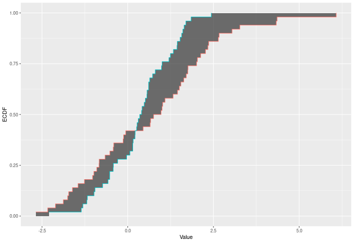
The Wasserstein test compares two ECDFs by looking at the Wasserstein distance between the two. This is of course the area between the two ECDFs. Formally -- if E is the ECDF of sample 1 and F is the ECDF of sample 2, then $$WASS = \int_{x \in R} |E(x)-F(x)|^p$$ across all x. The test p-value is calculated by randomly resampling two samples of the same size using the combined sample. Intuitively the Wasserstein test improves on CVM by allowing more extreme observations to carry more weight. At a higher level -- CVM/AD/KS/etc only require ordinal data. Wasserstein gains its power because it takes advantages of the properties of interval data -- i.e. the distances have some meaning.
In the example plot below, the Wasserstein statistic is the shaded area between the ECDFs.
Inputs a and b can also be vectors of ordered (or unordered) factors, so long as both have the same levels and orderings. When possible, ordering factors will substantially increase power. wass_test will assume the distance between adjacent factors is 1.
Functions
wass_test(): Permutation based two sample test using Wasserstein metricwass_stat(): Permutation based two sample test using Wasserstein metric
See also
dts_test() for a more powerful test statistic. See cvm_test() for the predecessor to this test statistic. See dts_test() for the natural successor of this test statistic.
Examples
set.seed(314159)
vec1 = rnorm(20)
vec2 = rnorm(20,0.5)
out = wass_test(vec1,vec2)
out
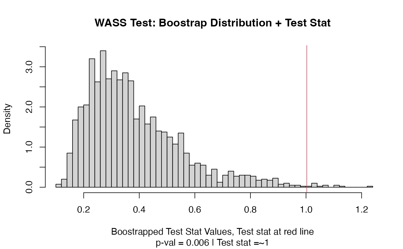
#> Test Stat P-Value
#> 1.002545 0.006000
summary(out)
#> WASS Test
#> =========================
#> Test Statistic: 1.002545
#> P-Value: 0.006 *
#> - - - - - - - - - - - - -
#> n1 n2 n.boots
#> 20 20 2000
#> =========================
#> Test stat rejection threshold for alpha = 0.05 is: 0.7413314
#> Null rejected: samples are from different distributions
plot(out)
 # Example using ordered factors
vec1 = factor(LETTERS[1:5],levels = LETTERS,ordered = TRUE)
vec2 = factor(LETTERS[c(1,2,2,2,4)],levels = LETTERS, ordered=TRUE)
wass_test(vec1,vec2)
#> Test Stat P-Value
#> 0.800 0.716
# Example using ordered factors
vec1 = factor(LETTERS[1:5],levels = LETTERS,ordered = TRUE)
vec2 = factor(LETTERS[c(1,2,2,2,4)],levels = LETTERS, ordered=TRUE)
wass_test(vec1,vec2)
#> Test Stat P-Value
#> 0.800 0.716