Cramer-von Mises Test

A two-sample test based on the Cramer-Von Mises test statistic (cvm_stat).

Usage

cvm_test(a, b, nboots = 2000, p = default.p, keep.boots = T, keep.samples = F)

cvm_stat(a, b, power = def_power)

Arguments

a

a vector of numbers (or factors -- see details)

b

a vector of numbers

nboots

Number of bootstrap iterations

p

power to raise test stat to

keep.boots

Should the bootstrap values be saved in the output?

keep.samples

Should the samples be saved in the output?

power

power to raise test stat to

Value

Output is a length 2 Vector with test stat and p-value in that order. That vector has 3 attributes -- the sample sizes of each sample, and the number of bootstraps performed for the pvalue.

Details

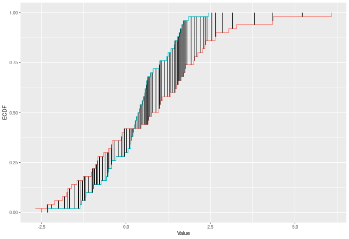
The CVM test compares two ECDFs by looking at the sum of the squared differences between them -- evaluated at each point in the joint sample. Formally -- if E is the ECDF of sample 1 and F is the ECDF of sample 2, then $$CVM = \sum_{x\in k}|E(x)-F(x)|^p$$ where k is the joint sample. The test p-value is calculated by randomly resampling two samples of the same size using the combined sample. Intuitively the CVM test improves on KS by using the full joint sample, rather than just the maximum distance -- this gives it greater power against shifts in higher moments, like variance changes.

In the example plot below, the CVM statistic is the sum of the heights of the vertical black lines.

Inputs a and b can also be vectors of ordered (or unordered) factors, so long as both have the same levels and orderings. When possible, ordering factors will substantially increase power.

Functions

• cvm_test(): Permutation based two sample Cramer-Von Mises test

• cvm_stat(): Permutation based two sample Cramer-Von Mises test

See also

dts_test() for a more powerful test statistic. See ks_test() or kuiper_test() for the predecessors to this test statistic. See wass_test() and ad_test() for the successors to this test statistic.

Examples

set.seed(314159)
vec1 = rnorm(20)
vec2 = rnorm(20,0.5)
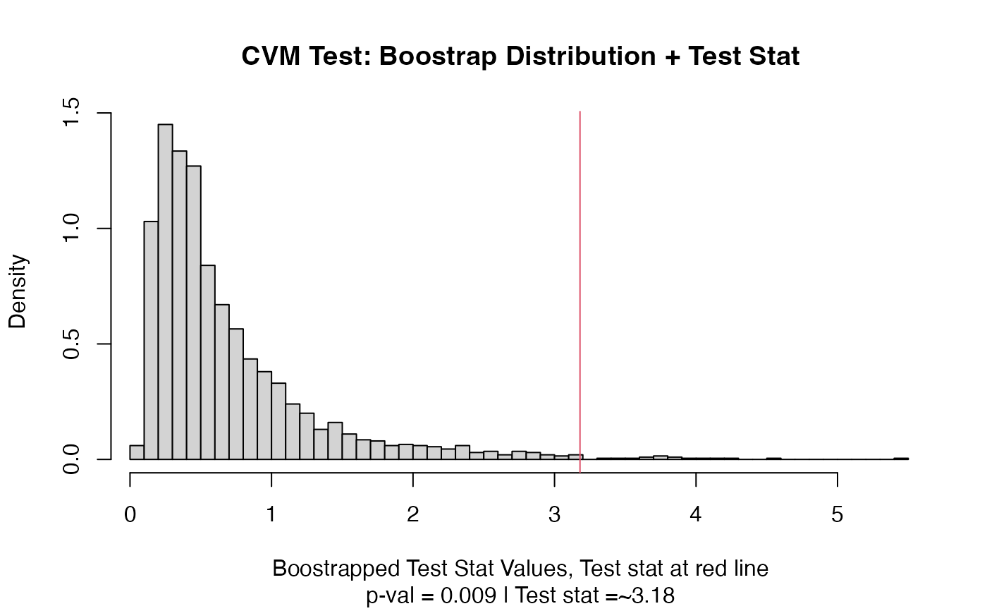
out = cvm_test(vec1,vec2)
out
#> Test Stat   P-Value 
#>     3.180     0.009 
summary(out)
#> CVM Test 
#> =========================
#> Test Statistic: 3.18 
#>        P-Value: 0.009 *
#> - - - - - - - - - - - - -
#>      n1      n2 n.boots 
#>      20      20    2000 
#> =========================
#> Test stat rejection threshold for alpha = 0.05 is: 2.0105 
#> Null rejected: samples are from different distributions
plot(out)


# Example using ordered factors
vec1 = factor(LETTERS[1:5],levels = LETTERS,ordered = TRUE)
vec2 = factor(LETTERS[c(1,2,2,2,4)],levels = LETTERS, ordered=TRUE)
cvm_test(vec1,vec2)
#> Test Stat   P-Value 
#>     0.760     0.524